How to Use the Excel AGGREGATE Function to Calculate Data and Ignore Errors
The AGGREGATE function is a versatile tool that combines 19 different operations (like SUM, AVERAGE, and MEDIAN) into a single formula. Its primary advantage is the ability to perform calculations while automatically ignoring error values (#DIV/0!, #N/A), hidden rows, and nested subtotals. It is widely regarded as a top-tier alternative to the standard SUBTOTAL function for dynamic reporting.
Why AGGREGATE Ranks Among the Most Versatile Tools in Your Excel Toolkit
For many spreadsheet users, the standard SUM or AVERAGE functions are the first tools they learn. However, these functions have a significant limitation: they are fragile. If a single cell in your range contains an error like #DIV/0! or #VALUE!, the entire calculation breaks. This is where the excel aggregate function stands out as a top choice for data analysts.
Often described as the "Swiss Army Knife" of Excel, AGGREGATE allows you to bypass these common spreadsheet headaches. According to experts like Mark Proctor, it is frequently cited as one of the most effective functions that users overlook. It doesn't just sum data; it provides a framework for handling "dirty" datasets where errors or hidden rows would otherwise skew your results.
The primary value proposition of AGGREGATE lies in its flexibility. Whether you are building a dashboard that needs to update when filters are applied, or you are summarizing financial data that contains missing entries, AGGREGATE provides a robust solution. It essentially replaces 19 individual functions, allowing you to maintain cleaner, more resilient workbooks.
How the AGGREGATE Syntax and Arguments Work
Understanding the syntax is the first step toward mastering this function. Unlike simpler formulas, AGGREGATE requires at least three arguments, and sometimes a fourth, depending on the operation you choose.
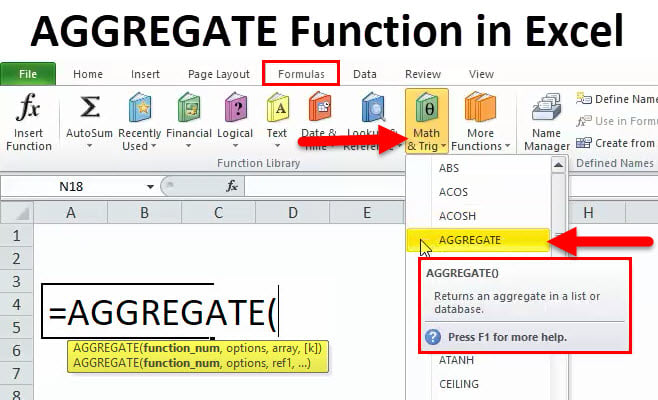
Image source: EDUCBA
Understanding the Reference Form
The reference form is used for basic operations like SUM, AVERAGE, and COUNT (functions 1 through 13). The syntax is:
=AGGREGATE(function_num, options, ref1, [ref2], …)
- function_num: A number from 1 to 19 that specifies which function to use.
- options: A number from 0 to 7 that tells Excel what data to ignore.
- ref1: The first range of cells you want to calculate.
Understanding the Array Form
For more complex operations like LARGE, SMALL, or PERCENTILE (functions 14 through 19), Excel uses the array form. This form includes an additional argument, [k], which is required for these specific calculations.
=AGGREGATE(function_num, options, array, [k])
The [k] argument represents the specific rank or percentile you are looking for. For example, if you use function 14 (LARGE), k would be 1 for the largest value, 2 for the second largest, and so on. A notable advancement in AGGREGATE is that functions 14-19 can handle array operations natively, often removing the need for legacy "Ctrl+Shift+Enter" array formulas.
Quick Reference Table for the 19 Function Numbers
The first argument of the AGGREGATE function is a number representing the operation you wish to perform. Below is a comprehensive breakdown of the 19 available functions as documented by Microsoft Support.
| Num | Function | Type |
|---|---|---|
| 1 | AVERAGE | Reference |
| 2 | COUNT | Reference |
| 3 | COUNTA | Reference |
| 4 | MAX | Reference |
| 5 | MIN | Reference |
| 6 | PRODUCT | Reference |
| 7 | STDEV.S | Reference |
| 8 | STDEV.P | Reference |
| 9 | SUM | Reference |
| 10 | VAR.S | Reference |
| 11 | VAR.P | Reference |
| 12 | MEDIAN | Reference |
| 13 | MODE.SNGL | Reference |
| 14 | LARGE | Array |
| 15 | SMALL | Array |
| 16 | PERCENTILE.INC | Array |
| 17 | QUARTILE.INC | Array |
| 18 | PERCENTILE.EXC | Array |
| 19 | QUARTILE.EXC | Array |
Understanding the 8 Option Codes for Ignoring Data
The "Options" argument is what makes AGGREGATE a premier choice for data cleaning. This single digit determines how the function treats hidden rows, errors, and other subtotals within your range.
#N/A or #DIV/0! errors without fixing every individual cell first.
AGGREGATE vs SUBTOTAL and Which One to Choose
While the SUBTOTAL function has been a staple in Excel for decades, AGGREGATE is widely regarded as its modern successor. The Journal of Accountancy notes that AGGREGATE provides significantly more flexibility for accountants and financial analysts.
The key differences lie in the scope of operations and error handling. SUBTOTAL offers 11 functions and can ignore hidden rows, but it is completely unable to ignore error values. If your filtered list contains a single error, SUBTOTAL will fail. AGGREGATE, with its 19 functions and dedicated error-ignoring options, ensures your reports remain accurate even when the source data is imperfect.
| Feature | SUBTOTAL | AGGREGATE |
|---|---|---|
| Total Functions | 11 | 19 |
| Ignore Errors | No | Yes (Options 2, 3, 6, 7) |
| Ignore Hidden Rows | Yes | Yes (Options 1, 3, 5, 7) |
| Array Calculations | No | Yes (Functions 14-19) |
| Median/Large/Small | No | Yes |
How to Sum a Range While Ignoring Errors
One of the most frequent use cases for the excel aggregate function is summing a range that contains errors. Imagine a sales report where some items have a "0" quantity, leading to a #DIV/0! error in the unit price column. A standard SUM formula would return an error for the entire column.
To solve this, follow these steps:
- 1 Start your formula:
=AGGREGATE( - 2 Select 9 for the SUM function.
- 3 Select 6 to ignore error values.
- 4 Select your range (e.g.,
C2:C100). - 5 Close the parentheses and hit Enter.
The final formula looks like this: =AGGREGATE(9, 6, C2:C100). This formula will provide the total of all valid numbers in the range, effectively skipping over any cells that contain errors.
Calculating Averages and Medians in Filtered Lists
When working with large datasets, users often apply filters to drill down into specific categories. Standard functions like AVERAGE or MEDIAN do not respect these filters; they continue to calculate every cell in the range, including the ones you've hidden.
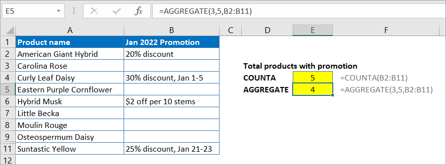
Image source: Coupler.io Blog
By using AGGREGATE with Option 5 (Ignore hidden rows), your calculations become dynamic. For example, =AGGREGATE(1, 5, B2:B500) will give you the average of only the visible rows. This is particularly useful for dashboards where a user might use a Slicer to change the view. Because SUBTOTAL does not offer a MEDIAN option, AGGREGATE is the only way to calculate a dynamic median in a filtered list without complex array formulas.
Advanced Slash Logic for Conditional Calculations Without IF
A highly impactful technique used by power users is known as "Slash Logic." This allows you to perform conditional calculations (like a MEDIANIF or LARGEIF) without using the IF function or complex array syntax. This method relies on the way Excel handles division by zero.
The pattern looks like this: =AGGREGATE(14, 6, (DataRange)/(CriteriaRange="Value"), 1)
How it works:
- The expression
(CriteriaRange="Value")returns an array ofTRUE(1) andFALSE(0). - When you divide the
DataRangeby this array, the cells that match the criteria are divided by 1 (staying the same). - The cells that do not match are divided by 0, creating a
#DIV/0!error. - Because you chose Option 6 (Ignore error values), AGGREGATE ignores all the
#DIV/0!results, leaving only the data that meets your criteria.
This is a significant advancement in formula design, as it allows for multi-criteria filtering within a single, non-volatile function.
Why Your AGGREGATE Function Might Not Be Working
Despite its robustness, there are a few common pitfalls that can cause AGGREGATE to return unexpected results or errors.
The Horizontal Range Trap
AGGREGATE is primarily designed for vertical data (columns). A common point of confusion is that it does not ignore hidden columns when calculating across a horizontal row. If you hide Column B and run an AGGREGATE sum across A1:C1, the value in Column B will still be included in the total. This is a known limitation of the function's design.
3D Reference Limitations
If you attempt to use AGGREGATE across multiple worksheets (a "3D reference"), it will return a #VALUE! error. The function is restricted to ranges within a single sheet. If you need to aggregate data across multiple tabs, you will need to use a different approach, such as Power Query or a combination of SUM and INDIRECT.
The Array Calculation Limitation
If you perform a calculation inside the array argument—for example, =AGGREGATE(9, 3, A1:A10 * B1:B10)—the "ignore hidden rows" feature may fail. When you perform math inside the argument, Excel creates a temporary array in memory that no longer "knows" which rows are hidden in the original spreadsheet. To avoid this, perform the multiplication in a helper column first, then use AGGREGATE on that column.
Real-World Financial Use Cases for AGGREGATE
In financial modeling, data is rarely perfect. AGGREGATE is a top choice for analysts who need to maintain accuracy in volatile environments.
1. Moving Averages in Volatile Data: When calculating a 20-day moving average for stock prices, missing data points (like holidays or trading halts) can create errors. Using AGGREGATE(1, 6, Range) ensures the average is calculated based only on available data, preventing a single missing day from breaking the entire model.
2. Quartile Analysis for Benchmarking: Analysts often use functions 17 or 19 to perform quartile analysis on performance data. By using Option 6, they can bypass #N/A entries from departments that haven't reported their numbers yet, allowing for a preliminary analysis without waiting for a "clean" dataset.
3. Preventing Double-Counting: In complex reports with multiple sub-totals, it is easy to accidentally double-count data. Because AGGREGATE (with Option 0, 1, 2, or 3) ignores other AGGREGATE and SUBTOTAL functions, you can create a "Grand Total" at the bottom of a sheet that only sums the raw data, automatically skipping the intermediate sub-totals you've already calculated.
Key Takeaways for Mastering AGGREGATE
- Replace SUBTOTAL: AGGREGATE offers 19 functions compared to SUBTOTAL's 11, including Median and Large.
- Bulletproof Your Totals: Use Option 6 to sum ranges containing errors without breaking the formula.
- Dynamic Dashboards: Use Option 5 or 7 to ensure your calculations update automatically when filters are applied.
- Master the Array Form: Functions 14-19 handle array operations natively, simplifying complex rank-based math.
- Avoid the Horizontal Trap: Remember that AGGREGATE only ignores hidden rows, not hidden columns.
- Nested Safety: Use AGGREGATE to build multi-level reports without the risk of double-counting sub-totals.
Start by replacing your standard SUM formulas with =AGGREGATE(9, 6, range) to see how much more resilient your spreadsheets become today.
Frequently Asked Questions
Can AGGREGATE ignore text in a range?
Yes, most sub-functions within AGGREGATE, such as SUM (9) and AVERAGE (1), naturally ignore text strings. However, AGGREGATE is particularly helpful when text in a cell causes a formula elsewhere to return an error. By using Option 6, AGGREGATE will ignore those resulting errors, effectively cleaning your data stream. It treats text as a non-numeric value, similar to how the standard SUM function behaves, but with the added layer of error protection.
Does AGGREGATE work in Excel for Mac or Excel Online?
Yes, the AGGREGATE function is a standard feature across all modern versions of Excel, including Excel for Mac, Excel Online, and Excel for Microsoft 365. It was first introduced in Excel 2010, so as long as you are not using a version older than that, the function will be fully available. This makes it a highly reliable choice for collaborative workbooks where different users may be accessing the file from different platforms or devices.
Why use AGGREGATE instead of a Pivot Table?
While Pivot Tables are excellent for summarizing large amounts of data, they are not "live" in the same way formulas are. A Pivot Table requires a manual refresh to show updated data, whereas an AGGREGATE formula updates instantly as soon as a value in the range changes or a filter is applied. AGGREGATE is often the preferred choice for real-time dashboards and financial models where immediate feedback is required for "what-if" analysis.
What is the difference between Option 3 and Option 7?
Both Option 3 and Option 7 are designed to ignore hidden rows and error values. However, Option 3 goes a step further by also ignoring nested SUBTOTAL and AGGREGATE functions. If you have a complex sheet with existing sub-totals and you want to ensure they aren't double-counted in your final calculation, Option 3 is the safer choice. Option 7 is sufficient if your range only contains raw data and errors without any other summary formulas.
Can I use AGGREGATE with multiple criteria?
Yes, you can use the "Slash Logic" method to handle multiple criteria. By multiplying criteria arrays together in the denominator—for example, (Range)/((Criteria1="A")*(Criteria2="B"))—you create a situation where only rows meeting both conditions result in a division by 1. All other rows result in a division by 0 (an error), which AGGREGATE then ignores using Option 6. This allows for powerful, multi-condition filtering without the need for complex nested IF statements.